Written by Jane Hames
This guide is aimed at Excel users who can already use the VLookup function and want to learn more about it. This is how to use the Excel Vlookup using TRUE
If you use a VLookup, the chances are you will use FALSE as the Range Lookup finding an exact match for the Lookup Value in the first column of your Table Array. I often get asked when you would use TRUE as your Range Lookup and this is good question as it’s not used half as often as FALSE.
Last week I was able help one of my Excel course delegates to solve a problem she had, and the solution to the problem was to use a Vlookup with TRUE. I wanted to share what we did with my readers and followers as it might give you some good ideas of things you could do with your own work. All data in the guide below is fictional, but based on the real world scenario:
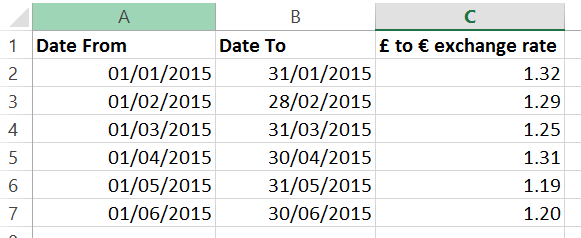
The scenario I was given, is that as shown in the image below, there are a list of date ranges with different exchange rates for different date ranges.
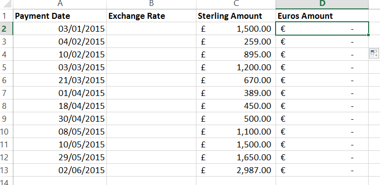
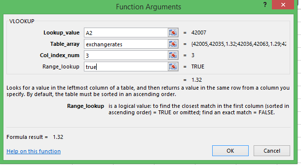
We wanted to ensure that the correct exchange rate was used to calculate the payment amount in Euros as shown in the image below: In order to do this, I used a Vlookup to pick up the correct exchange rate for the specified payment date. This payment date would need to sit in one of the date ranges listed. This is what we used to do this calculation:
LOOKUP_VALUE: The payment date 
TABLE_ARRAY: The table which shows the date ranges listed in ascending order (the Date From in the first column of the table_array is what Excel will use). The exchange rate is in the third column of the table_array.:
COL_INDEX_NUMBER: 3 This is the column in the table_array that contains the exchange rate we are looking for.
RANGE_LOOKUP: TRUE This ensures that Excel will look at the earliest date in the list that is close to the payment date (our lookup_value).
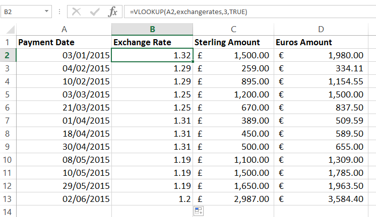
This what the formula looks like at the end:
Note that the payment date is shown as its reference number rather than the date. This is because I have selected SHOW FORMULAS in order to show you the formulae on the sheet. I then copied the formula down so that I have ended up with this end result:
If you would like help with the Vlookup or other functions in Excel, please get in touch.

