How to change PivotTable grouping in one table without affecting another table

Written by Jane Hames

This post is aimed at those who already use PivotTables (as many of my trainees do!).

PivotTable grouping is easy enough to do, but it could cause a lot of frustation if you want to change the grouping in one table without changing the way that field is grouped in another table.

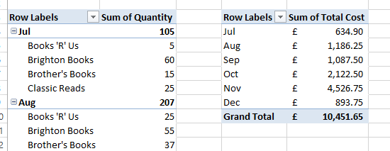
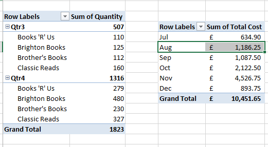
The image above shows my two PivotTables and in both, the individual dates have been grouped by month, using the Group Field feature.

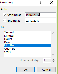
If I change the grouping from months to quarters in one PivotTable, it will also change in the other. This is because they are based on the same source data and therefore share the same cache.

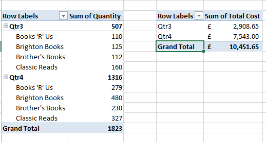
“HOW DO I GET IT TO WORK?” I hear you cry! You just need to do this:

1. Highlight the area of cells containing your second PivotTable and cut it (Ctrl X).



2. Go to a new workbook and paste it in (Ctrl V).
3. Change the grouping style on the second PivotTable that is now in a new workbook.



4. Cut this second PivotTable again from the new workbook and paste it into the original workbook.

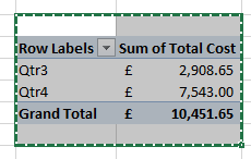
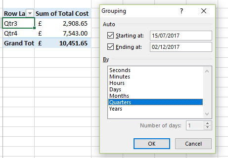
Both PivotTables are based on separate caches now, which means you can change the grouping in one PivotTable without affecting the other.

NOTE: This will increase the file size as we have double the amount of data due to the separate caches. As always, there are several ways to get to an end result in Excel, I find this method is very quick and easy (when you know how!).

If you or your team would benefit from being briliant at PivotTables, please do get in touch.