Written by Jane Hames
PivotTables are one of Excel’s most powerful tools, designed to make data analysis quick & easy. This How-To Guide is aimed at those who already use PivotTables and want to learn some new techniques.
In a PivotTable you can apply filters to your data using the report filter and by filtering within the row or column fields. When using multiple items in a report filter it is not obvious which criteria you have specified and likewise with the row and column filters. So what can you do?
The answer is to use Slicers in Excel 2010 and this is how to do it:
- Ensure that you are not working in compatibility mode. (If you are, convert your workbook first.)
- Refresh the PivotTable by clicking on the Refresh button on the PivotTable tools, Options tab.
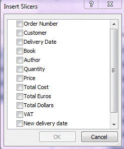
- Click on the Insert Slicer button and select Insert Slicer.
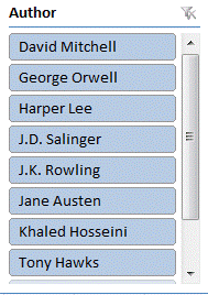
- Tick the fields you want to use to filter with, and a Slicer box will be displayed with items in the fields.
- Specify your criteria by clicking on the item, or hold the Ctrl key and click to select more than one. The PivotTable will change to show only the data meeting your criteria.
- To clear a Slicer filter, click on the clear filter button in the top right of the slicer box.
- To remove a slicer box, click on the edge of the box and press Delete on the keyboard.